Interest Rate Theory

Visual overview

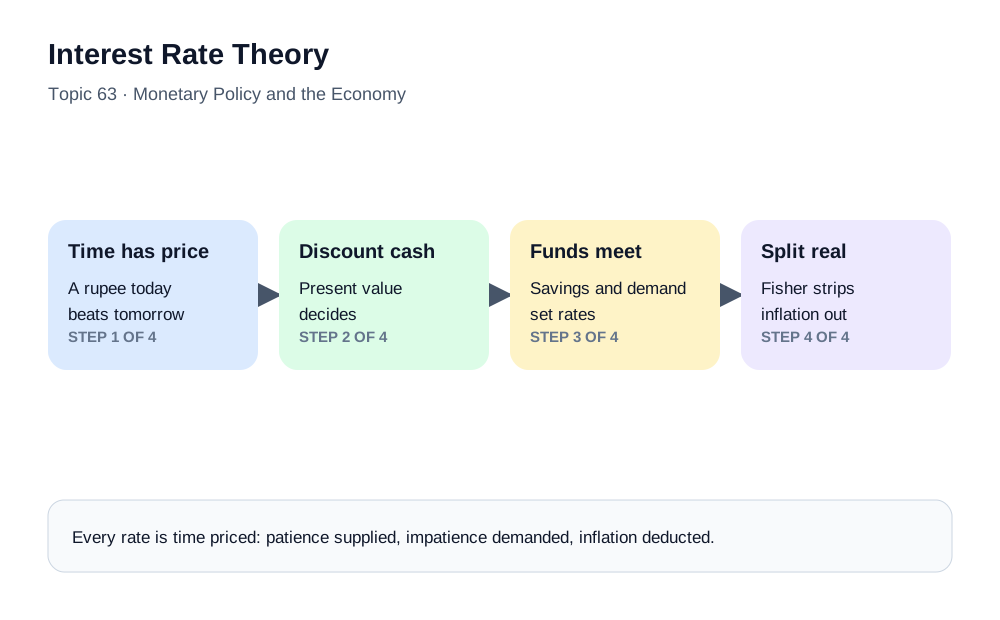
Interest Rate Theory at a glance — Time value of money, term structure, Fisher Effect.

The Price of Money Through Time

Interest rates function as the fundamental pricing mechanism for money across time, representing both the cost of borrowing and the reward for deferring consumption. In banking, interest rates determine what institutions earn on their assets, what they pay for their liabilities, and ultimately whether their operations prove profitable or loss-making. Behind the specific rates quoted on loan documents and deposit statements lies a sophisticated theoretical framework explaining why money possesses time value, how rates are determined in different market segments, and what factors cause them to change over time. Mastering these theoretical foundations enables banking professionals to anticipate rate movements, manage interest rate risk, and make informed pricing decisions across diverse product categories.

This chapter builds that framework from first principles to the asset-liability desk. By the end you will be able to:

• Explain the time value of money and compute present values.
• Compare the loanable funds and liquidity preference theories of rate determination.
• Decompose nominal rates into real rates and inflation expectations via the Fisher effect.
• Explain the term structure's competing theories and read yield curve shapes.
• Describe the benchmark transition from LIBOR to risk-free rates.
• Measure interest rate risk through gap and duration analysis.
• Connect rate theory to net interest margin — and to the 2023 bank failures.

1. First Principles: The Time Value of Money

The time value of money represents one of the most fundamental principles in all of finance, stating unequivocally that a dollar available today holds greater value than a dollar promised at some future date. This principle rests upon several robust foundations of human behavior and economic reality. Consumption preference reflects the natural human tendency to prefer present gratification over future benefits, meaning individuals require compensation to postpone consumption to future periods. Inflation systematically erodes the purchasing power of money over time, so future dollars buy fewer goods and services than current dollars, necessitating nominal returns that preserve or enhance real purchasing power. Risk pervades all future promises, as uncertainty about whether promised payments will actually materialize requires compensation for bearing that uncertainty. Opportunity cost captures the returns forgone by holding cash rather than investing it productively, establishing a minimum required return for any capital commitment. Together these factors create the theoretical underpinning for positive interest rates in normally functioning economies.

The interest rate, seen this way, is not one price but a stack of compensations: payment for waiting, payment for expected inflation, payment for the chance of not being paid, and payment for the alternatives forgone. Every quoted rate in banking — from a savings account to a thirty-year mortgage — is some combination of these layers, and learning to see the layers is the beginning of rate literacy. Negative nominal interest rates, which have occurred in several monetary systems, do not invalidate time-value-of-money logic. They can arise when monetary-policy settings, demand for safe and liquid assets, institutional constraints, inflation expectations, and the costs or inconvenience of holding physical cash make investors willing to accept a small negative nominal return for particular assets. The result is better understood through the full monetary and portfolio framework than as a central bank simply 'overwhelming' a natural positive rate.

2. Present Value: The Mathematics of Time

The present value formula provides the mathematical machinery for comparing cash flows occurring at different times, enabling financial decision-makers to translate future amounts into equivalent present values using an appropriate discount rate. The formula expresses present value as future value divided by one plus the interest rate raised to the power of the number of periods. This seemingly simple equation underlies virtually all financial valuation, from mortgage pricing to corporate investment analysis to derivatives valuation. Small changes in the discount rate assumption produce substantial present value differences for distant cash flows, explaining why long-duration assets such as thirty-year bonds exhibit such sensitivity to interest rate movements and why banks carefully manage the duration mismatch between their assets and liabilities.

A worked example makes the sensitivity tangible. A payment of one thousand due in one year, discounted at five percent, is worth about nine hundred fifty-two today. The same payment due in thirty years at five percent is worth about two hundred thirty-one. Now move the discount rate from five to seven percent: the one-year payment loses about two percent of its present value, but the thirty-year payment falls to about one hundred thirty-one — a forty-three percent loss. This is the mathematics underneath everything that follows: the further away the cash flow, the more violently its value swings when rates move. Bond duration, bank balance sheet risk, and the 2023 banking failures are all, at root, this single equation operating at scale.

3. Loanable Funds: The Real Economy's Rate

Several competing but complementary theories explain the determination of interest rates in different economic contexts. The classical theory of loanable funds conceptualizes the interest rate as the market-clearing price that equilibrates the supply of savings from households and institutions with the demand for investment from businesses and governments. According to this framework, anything that increases the propensity to save, such as demographic shifts toward prime saving years or increased uncertainty about future needs, will increase the supply of loanable funds and exert downward pressure on interest rates. Conversely, anything that increases investment demand, such as technological innovations that raise expected returns on capital or expansionary fiscal policy that increases government borrowing, will raise interest rates by increasing demand for loanable funds. This framework emphasizes real factors of saving and investment in determining interest rates, with monetary forces operating primarily through their effects on these real decisions.

The loanable funds lens explains the long trends that central banks do not control: the decades-long decline of real interest rates across advanced economies, attributed to aging populations saving more, businesses needing less physical capital, and a global glut of savings seeking safe assets. When analysts say "rates are low for structural reasons," they are speaking loanable funds. The fiscal chapter's crowding-out mechanism is also this theory in action: government borrowing is investment demand, and its pressure on rates depends on how much slack the saving-investment balance has.

4. Liquidity Preference: The Monetary Rate

Keynesian liquidity preference theory offers an alternative perspective emphasizing monetary factors and the special role of money as the most liquid asset. According to this framework, interest represents the reward for parting with liquidity and holding less liquid interest-bearing assets instead of money. The demand for money arises from three distinct motives: the transactions motive reflecting the need for money to facilitate regular payments, the precautionary motive reflecting the desire to hold reserves against unexpected contingencies, and the speculative motive reflecting portfolio allocation between money and bonds based on interest rate expectations. When interest rates are low, the opportunity cost of holding money is small, so liquidity preference is high and bond prices are bid up to the point where expected capital losses offset current yield. When interest rates are high, the reward for holding bonds rather than money is substantial, encouraging portfolio shifts away from money. The central bank influences interest rates through its control of money supply, with expansionary policy reducing rates and contractionary policy raising them.

The two theories are complements with different time horizons: liquidity preference governs the short end, where central bank policy dominates and the money markets chapter's machinery operates; loanable funds governs the long run, where saving and investment fundamentals assert themselves. A complete rate view holds both: the central bank steers overnight money, but the thirty-year rate ultimately answers to demographics, productivity, and fiscal trajectories — which is why long rates sometimes move opposite to the policy rate when the fundamentals overwhelm the steering.

5. The Fisher Effect: Splitting Nominal from Real

The Fisher Effect establishes the crucial relationship between nominal interest rates, real interest rates, and inflation expectations. The nominal rate observed in markets represents approximately the sum of the underlying real rate and expected inflation over the relevant period. This decomposition matters enormously for both borrowers and lenders, as it is the real rate that determines actual changes in purchasing power. If expected inflation rises by two percentage points, nominal rates should eventually rise by a similar amount to leave real rates unchanged, though this adjustment may occur with lags depending on contractual arrangements and market expectations. The Fisher Effect explains why inflation-targeting central banks focus on real interest rates when assessing policy stance and why long-term nominal rates incorporate substantial inflation risk premiums when inflation uncertainty is high.

The previous chapter worked the arithmetic from the saver's perspective; here the theoretical point is the decomposition itself. Every nominal rate contains an inflation forecast. When the central bank assesses whether policy is "tight" or "loose," it compares the real rate — nominal minus expected inflation — against the economy's neutral rate, the real rate consistent with stable inflation. A nominal rate of five percent can be restrictive or stimulative depending entirely on whether expected inflation is two percent or six: same number, opposite stance. This is why sophisticated rate analysis never quotes a nominal rate without its inflation context.

6. The Term Structure: Why Maturity Has a Price

The term structure of interest rates describes how yields vary across different maturity horizons for otherwise comparable securities, giving rise to the yield curve that plots yields against time to maturity. Several theories explain the shape and behavior of the yield curve. Pure expectations theory posits that long-term rates represent the average of expected future short-term rates over the relevant horizon, implying that investors are indifferent to maturity and seek only the highest expected return. The liquidity premium theory modifies this view by recognizing that longer maturities expose investors to greater interest rate risk, for which they demand compensation in the form of higher yields, causing the yield curve to slope upward even when rate expectations are stable. The segmented markets theory suggests that supply and demand conditions differ across maturity segments due to institutional preferences and regulatory requirements, with each segment determined independently. The preferred habitat theory offers a middle ground, acknowledging that investors have maturity preferences but will shift to other segments if yield differentials provide sufficient compensation.

The theories answer different questions, and practitioners use them all. Expectations theory explains curve movements: when the two-year yield jumps after a central bank surprise, markets are repricing the policy path. Liquidity premium explains the curve's default tilt: upward slope as compensation for duration risk. Segmentation and preferred habitat explain anomalies: pension fund demand compressing long yields, treasury bill issuance shifting the short end, the kinks that pure expectations cannot produce. The bond markets chapter applies the shapes to macro signals; here the theoretical toolkit is what lets you say why the curve looks as it does.

7. Reading the Curve: Signals and Margins

The yield curve shape conveys important information about market expectations and economic conditions. A normal upward-sloping curve indicates that markets expect continued growth and that investors demand higher yields for assuming the greater risks of longer maturities. A flat yield curve suggests uncertainty about future economic conditions, with short and long rates converging as expectations become muddled. An inverted yield curve, where selected short-term yields exceed longer-term yields, has historically been associated with elevated recession risk in several markets, but it is an indicator rather than a deterministic forecasting rule. The curve reflects expected future policy rates together with term premia, inflation expectations, supply-demand effects, and market-specific factors. A steep curve can accompany expected recovery or rising inflation and term premia, among other conditions. Banks monitor curve shape because it affects asset pricing, funding, reinvestment, hedging, and customer behaviour, but a bank's net interest margin cannot be inferred from slope alone: deposit beta, asset repricing, product spreads, hedges, and behavioural maturities can dominate the simple 'borrow short and lend long' story.

The bank's relationship with the curve is structural, not incidental. Banking's core business model — borrow short, lend long — is a leveraged position on the curve's upward slope. When the curve is steep, the transformation earns handsomely; when flat, the margin thins; when inverted, the model runs at a structural loss on new business, and banks compensate with fees, credit spread, and volume. This is why an inverted curve forecasts more than recession: it forecasts a banking profitability squeeze arriving first, a point examiners and interviewers both know.

8. Benchmarks: From LIBOR to Risk-Free Rates

Interest rate benchmarks provide the reference points upon which trillions of dollars of financial contracts depend, making their integrity and reliability matters of systemic importance. The London Interbank Offered Rate, or LIBOR, dominated global finance for decades as the reference rate for everything from corporate loans to derivatives to residential mortgages. LIBOR represented estimated borrowing costs reported by panel banks rather than actual transaction rates, a methodology that proved vulnerable to manipulation during the 2008 financial crisis and its aftermath. Regulatory investigations revealed serious misconduct in LIBOR submissions, while the decline in underlying unsecured term-bank borrowing also undermined the benchmark's long-term robustness. Most non-US-dollar LIBOR panels and certain US-dollar settings ended after 2021, the remaining US-dollar panel settings ceased at end-June 2023, and temporary synthetic settings used for limited legacy purposes ceased subsequently. The final remaining synthetic US-dollar LIBOR settings were published for the last time on 30 September 2024, after which LIBOR had fully ceased. The transition to alternative reference rates based on actual overnight transactions rather than bank estimates represents one of the most consequential changes in financial market infrastructure in generations.

Major LIBOR currencies transitioned toward more robust reference-rate frameworks, including SOFR in US dollars, SONIA in sterling, €STR in euro markets, and TONA in Japanese yen. These risk-free or near-risk-free overnight benchmarks are grounded more directly in transaction data than LIBOR's panel-bank term methodology. Markets use overnight compounding, backward-looking realised rates, and in some cases approved or recognised term constructions depending on product and jurisdiction. India has its own benchmark architecture, including MIBOR for the domestic overnight money market, but MIBOR should not be presented as though it were simply another currency-specific LIBOR successor created by the global LIBOR transition.

The money markets chapter tells the full transition story; the theoretical consequence belongs here. LIBOR was a term rate embedding bank credit risk — it rose when banks' creditworthiness fell, automatically building stress into loan pricing. The risk-free rates embed almost no credit risk, so the new architecture prices bank credit separately, as an explicit spread. The change altered how floating-rate contracts behave in crises: under LIBOR, a bank borrower's rate rose when the banking system wobbled; under SOFR, it does not — unless the credit spread is explicitly adjusted. The theory of what a benchmark contains turns out to matter as much as its level.

9. Interest Rate Risk: Banking's Structural Exposure

Interest rate risk management constitutes a critical function for banking institutions given their fundamental business model of maturity transformation. Banks typically fund themselves through short-term deposits and similar liabilities while making longer-term loans and investments, creating an inherent duration mismatch that exposes them to interest rate movements. When rates rise, the cost of funding increases more quickly than the income from fixed-rate assets, squeezing net interest margins. When rates fall, income from floating-rate loans declines while funding costs may remain sticky, again pressuring margins. Asset-liability management seeks to control these exposures through careful matching of asset and liability durations, interest rate derivatives hedging, and strategic positioning based on interest rate outlook.

The mismatch is not a flaw to be eliminated — it is the business itself. Banks are paid to transform short money into long credit; the skill lies in holding the transformation within bounds the institution can survive. The toolkit includes natural hedging (matching fixed-rate loans with fixed-rate funding), derivatives (interest rate swaps converting fixed to floating exposure, covered in the derivatives chapter), product design (floors on floating loans, caps on deposit rates), and strategic positioning (deliberately running a measured gap in the direction of the rate view). Every one of these choices is interest rate theory applied as risk management.

10. Gap Analysis and Duration: Measuring the Exposure

Gap analysis provides a fundamental tool for measuring interest rate risk exposure, categorizing assets and liabilities by their repricing time buckets and calculating mismatches within each bucket. A negative gap in short-term buckets, where rate-sensitive liabilities exceed rate-sensitive assets, indicates vulnerability to rising rates, as funding costs would increase faster than asset yields. A positive gap indicates the opposite exposure, benefiting from rising rates but suffering when rates decline. Duration gap analysis extends this approach by considering the weighted average time until cash flows are received or paid, providing a more comprehensive measure of interest rate sensitivity. Net interest margin at risk quantifies the potential impact of specified interest rate shocks on earnings, informing both tactical positioning and strategic decisions about balance sheet structure.

A miniature balance sheet shows the arithmetic. Suppose a bank holds sixty billion of rate-sensitive assets repricing within one year against eighty billion of rate-sensitive liabilities repricing within the same window: a negative one-year gap of twenty billion. A one percentage point rise in rates then costs roughly two hundred million of annual net interest income as the extra twenty billion of liabilities reprices upward with no offsetting asset income. Duration gap tells the longer story: if the bank's assets have an average duration of four years and liabilities of one, a one-point rate rise knocks roughly three percent off the economic value of equity — the balance sheet shrinks in real terms even where accounting masks it. The 2023 failures, examined below, were this arithmetic ignored.

11. Net Interest Margin: Where Theory Meets the P&L

Net interest margin, the spread between interest earned on assets and interest paid on liabilities expressed as a percentage of average earning assets, serves as the primary profitability metric for traditional banking operations. This margin reflects both market conditions, including the level and slope of the yield curve, and bank-specific factors such as credit risk pricing, funding mix, and operational efficiency. Managing NIM effectively requires not merely passing through policy rate changes to customers but also maintaining appropriate risk premiums, optimizing funding composition between deposits and wholesale sources, and continuously adjusting portfolio positioning as market conditions evolve.

Two levers dominate NIM management in practice. Deposit beta — the fraction of a policy rate change passed to depositors — determines liability costs: banks with sticky, loyal deposit bases keep betas low and margins wide when rates rise, while banks funded by rate-shopping wholesale money see costs chase assets upward. Asset repricing structure determines the other side: floating-rate loan books benefit immediately from hikes, fixed-rate books wait. NIM management through a rate cycle is therefore a forecasting exercise about two behaviors — depositors' patience and the loan book's clock speed — and the theories of this chapter are its working vocabulary.

12. Case Study: 2023 — When Duration Theory Failed a Bank

In March 2023, Silicon Valley Bank — a mid-sized American bank that had grown rapidly on technology-sector deposits — collapsed in forty-eight hours, and the autopsy is a pure application of this chapter. During the near-zero rate era, the bank placed a large share of its swelling deposits into long-dated, fixed-rate government and agency bonds yielding little but considered safe from default. Duration, not credit, was the risk taken: the bond portfolio's cash flows sat far in the future, precisely the configuration Section 2's present value mathematics makes most fragile.

When the central bank tightened at the fastest pace in decades, two repricings struck simultaneously. The bond portfolio's market value fell by billions as yields rose — duration theory operating exactly as the formula predicts — while the bank's deposit base, far from the loyal low-beta funding of NIM theory, proved to be concentrated, connected, and mobile: technology-sector depositors with uninsured balances withdrew at digital speed when losses became visible. The bank's attempt to raise capital to cover realized losses accelerated the run it was meant to stop; regulators closed it within days, and contagion fears spread to similar institutions.

The case is taught everywhere now because it compresses the whole syllabus: time value and duration (long assets, violent repricing), Fisher decomposition (nominal rates repricing to new inflation expectations), gap and duration gap (a negative economic position hidden by accounting categories), liquidity preference (funding is a behavior, not a balance), and the curve's banking squeeze. None of the theory failed in 2023 — the failure was running a balance sheet as if it did not apply.

13. Common Misconceptions About Interest Rate Theory

"The central bank sets 'the' interest rate." It sets one overnight policy rate; the economy's thousands of other rates emerge from expectations, risk, maturity, and credit layered on top. Long rates can rise while policy falls — the term structure has its own logic.

"A higher nominal rate always means tighter money." Only if it exceeds expected inflation by more than before. Six percent nominal with five percent expected inflation is looser than three percent with zero — the Fisher decomposition, not the headline number, defines the stance.

"Long-term rates predict the future." They aggregate expectations plus term premium plus segment demand. A low long rate may signal expected weakness, heavy pension buying, or both — reading forecasts off the curve requires knowing what else lives in it.

"Interest rate risk is a trading-desk problem." It is the banking book's central structural risk: maturity transformation is the business model, and 2023 proved that 'safe' government bonds can sink a bank through duration without a single default.

"Duration is just another word for maturity." Maturity counts time to the final payment; duration weights all cash flows by when they arrive. A thirty-year bond's duration might be fifteen years, and a zero-coupon bond's duration equals its maturity — the difference is exactly the interest rate sensitivity that matters.

"Bonds are safe if you hold them to maturity." Cash-flow-safe, yes; value- and liquidity-safe, no. Hold-to-maturity accounting records the fiction until forced sales make it fact — the distinction that separated survivors from failures in 2023.

"Negative rates prove time preference is dead." They prove policy can override natural compensations at the short end for a time. The decade of negative rates ended with the fastest normalization in modern memory — the theory's foundations outlasted the experiment.

14. Frequently Asked Questions

Why does money have time value? Because waiting costs: present consumption is preferred, inflation erodes future purchasing power, future payment is uncertain, and invested money earns. Interest is the price that compensates all four at once.

What is the difference between real and nominal interest rates? Nominal is the quoted rate; real is nominal minus expected inflation — the true change in purchasing power. All serious rate analysis works in real terms, because purchasing power is what economic decisions respond to.

What determines long-term interest rates? Expected future short rates (the policy path), plus term premium for duration risk, plus supply-demand conditions in each maturity segment — demographics, fiscal issuance, and institutional demand included. The central bank's grip weakens with maturity.

Why does the yield curve usually slope upward? Two forces: term premium compensating investors for the greater price risk of longer maturities, and (sometimes) expected rising rates. Even with flat rate expectations, the liquidity premium tilts the curve up.

What does an inverted yield curve mean for a bank? Structurally compressed margins: funding costs (short rates) exceed what new long-term lending earns. Banks respond with fee income, wider credit spreads, shorter asset duration, and hedging — and credit standards typically tighten, which is one way inversion helps produce the slowdown it predicts.

What replaced LIBOR and why does it matter? Overnight transaction-based risk-free rates — SOFR, SONIA, €STR, TONA, with MIBOR in India — chosen because estimate-based LIBOR was manipulable and increasingly hypothetical. The deeper change: benchmarks no longer embed bank credit risk, so crisis-era automatic repricing moved from the benchmark into explicit credit spreads.

What is duration, in one sentence? The weighted average timing of an instrument's cash flows — and therefore the multiplier translating a rate change into a price change: duration seven means roughly seven percent price move per one-point rate move.

How do banks measure interest rate risk? Gap analysis (repricing mismatches by time bucket), duration gap (economic value sensitivity of the whole balance sheet), and NIM-at-risk (earnings impact of specified rate shocks) — reported to regulators and steered by the asset-liability committee.

Why do interest rates differ so much between countries? Inflation expectations first (Fisher: high-inflation economies carry high nominal rates), then growth and investment returns (loanable funds), then currency and country risk premiums. Comparing nominal rates across countries without the inflation context compares nothing.

What is the difference between the policy rate and the neutral rate? The policy rate is what the central bank sets today; the neutral rate is the theoretical real rate at which the economy runs at capacity with stable inflation. Policy is tight or loose only relative to neutral — which is unobservable and must be estimated, one reason policy is judgment, not formula.

How do interest rate swaps reduce a bank's risk? By converting cash flow types: a bank receiving fixed loan payments can swap them for floating receipts, matching its floating funding and shrinking its duration gap — transforming exposure without selling a single loan, as the derivatives chapter details.

Can interest rates be negative, and what does that mean? Yes — several central banks set negative policy rates, effectively charging banks to hold reserves, aiming to spur lending and spending. It inverts the normal compensation logic deliberately and temporarily; savers still face mostly zero or positive retail rates because banks resist charging them outright.

15. Key Terms in This Chapter

• Time value of money — present money exceeds future money in value; interest is the price of the wait.
• Present value / discount rate — the machinery translating future cash flows into today's terms.
• Loanable funds theory — rates as the clearing price of saving supply and investment demand.
• Liquidity preference — rates as the reward for parting with money's liquidity; transactions, precautionary, speculative motives.
• Fisher effect — nominal rate ≈ real rate + expected inflation.
• Neutral rate — the real rate consistent with stable inflation; the stance yardstick.
• Term structure / yield curve — yields across maturities; its shape as signal and as bank-margin driver.
• Expectations / liquidity premium / segmented markets / preferred habitat — the term structure's explanatory theories.
• Term premium — extra yield for duration risk, above expected short rates.
• Benchmark / SOFR / SONIA / €STR / TONA / MIBOR — the post-LIBOR reference rates.
• Maturity transformation — borrowing short, lending long; banking's model and its structural risk.
• Gap analysis / duration gap — repricing-bucket and economic-value measures of rate exposure.
• Net interest margin (NIM) — asset yield minus funding cost over earning assets; banking's core profitability metric.
• Deposit beta — the fraction of rate changes passed to depositors.
• Interest rate swap — the derivative converting fixed to floating exposure; the hedger's main tool.
• Repricing bucket — a time band in gap analysis grouping items by when their rates reset.
• Rate-sensitive assets/liabilities — balance sheet items whose yields reset within the analysis window.
• NIM at risk — projected earnings impact of specified rate shocks.

16. Interview Insights: How This Topic Appears in Banking Interviews

"Explain why interest rates exist at all." Layered compensation: for waiting (time preference), for inflation erosion, for default uncertainty, for opportunities forgone. Candidates who decompose rather than recite — and who can then explain why a central bank might deliberately force the price negative — demonstrate theory as understanding.

"Nominal five percent: tight or loose?" Unanswerable without expected inflation — the Fisher point. Five minus two is restrictive; five minus five is neutral; five minus seven is stimulative. The question tests whether the candidate thinks in real terms, which is the dividing line between rate literacy and rate citation.

"Why did long-term rates fall for decades before 2022, and what changed?" Loanable funds: aging savers, capital-light investment, global savings glut compressing real rates. The change: inflation's return forcing nominal repricing, fiscal issuance expanding supply, and central banks shifting from buyers to sellers of duration. Holding both the structural and the cyclical story is the senior answer.

"Walk me through how a rate hike hits a bank's P&L." Funding costs reprice first (deposits by beta, wholesale instantly), floating assets follow, fixed assets lag; NIM's direction depends on the gap; bond portfolios take duration losses; credit costs arrive later as borrowers strain. Sequencing beats magnitude in the answer — the cycle has a script.

"What killed Silicon Valley Bank?" Duration mismatch on 'safe' long bonds, a concentrated mobile deposit base, hold-to-maturity accounting that concealed economic losses until a capital raise revealed them, and digital-speed liquidity. The meta-lesson: interest rate risk and liquidity risk are the same risk at different speeds — and both were textbook material all along.

"If you had to watch one number to understand rate conditions, what would it be?" A defensible pick: the two-year government yield, which concentrates the market's policy-path expectations with minimal term-premium noise — read alongside core inflation for the real-rate picture. The point of the question is not the ticker but the reasoning: choose the maturity that isolates expectations, and defend the choice.

Summary and Key Takeaways

• Interest is the price of money through time — layered compensation for waiting, inflation, risk, and forgone alternatives.
• Present value mathematics rules everything: distant cash flows swing violently with rates, which is duration, and duration is destiny for long-asset portfolios.
• Loanable funds explains structural rate trends (saving and investment); liquidity preference explains the short end the central bank steers; serious analysis holds both.
• The Fisher effect splits nominal from real — the stance of policy lives in the real rate, never the headline.
• The term structure blends expectations, term premium, and segment demand; the curve's shape is simultaneously a macro signal and the banking margin's script.
• LIBOR's replacement by overnight risk-free rates moved bank credit risk out of the benchmark and into explicit spreads — a subtle change with crisis-behavior consequences.
• Banking's business model is a leveraged position on rate theory: maturity transformation, gap and duration measurement, deposit betas, and NIM management are this chapter applied daily.
• 2023 proved the syllabus in forty-eight hours: duration risk and liquidity risk are one risk at two speeds, and no accounting category suspends the arithmetic.

Next: Topic 64 — Exchange Rate Systems →

Deep Dive: Turning Rate Theory Into Bank Pricing and Asset-Liability Decisions

Interest-rate theory becomes useful in banking when every quoted rate is decomposed into the risks and costs it is paying for. A customer sees one number. The bank sees a stack: reference rate or funding curve, liquidity cost, credit spread, capital charge, operating cost, optionality, product margin, and sometimes taxes or regulatory costs. Treasury then asks a second question: how will that rate behave when the yield curve changes and customers exercise their options?

The central practical lesson is that there is no single interest rate in an economy. There is a network of rates differentiated by maturity, currency, credit, collateral, liquidity, market structure, and contractual option. The policy rate anchors part of that network, but banks earn or lose money through the spreads and behavioural differences between its components.

The risk-free curve is a starting point, not a customer price

When a bank prices a loan, it needs a benchmark representing the time value and market cost of money in the relevant currency and maturity. That benchmark can come from government securities, swaps, overnight reference rates, or internal funds-transfer-pricing curves depending on the institution and product.

The customer rate then includes additional economics.

Suppose a five-year corporate loan is quoted at 8.5%. A simplified internal decomposition might be:

• matched-maturity funding or reference curve: 5.0%;
• liquidity and balance-sheet cost: 0.5%;
• expected credit loss: 0.8%;
• capital and operating cost: 0.7%;
• target return and relationship margin: 1.5%.

The exact components differ by bank, but the discipline matters. If the reference curve rises 100 basis points and the bank keeps the same customer price, it has silently given away margin unless some other component changed.

Credit spread and interest-rate risk should be separated

A bond or loan yield can rise because the risk-free curve rises or because the borrower's credit spread widens. Those are economically different events.

If a strong corporate bond yield increases from 6% to 7% entirely because government yields rose, the issuer's credit quality may be unchanged. If government yields remain stable but the corporate bond moves to 8%, the market is demanding more compensation for credit, liquidity, or other issuer-specific risk.

Bank risk systems therefore separate rate risk from spread risk. ALM manages structural interest-rate exposure. Credit and market-risk teams monitor changes in borrower and sector spreads. Combining them into one yield movement can hide the actual driver.

Discount curves and projection curves can differ

In derivatives and some floating-rate products, the curve used to project future cash flows can differ from the curve used to discount them. Modern collateralised derivatives markets developed multi-curve valuation frameworks because the funding and collateral economics of the instrument matter.

A business analyst working on a rates product should therefore avoid a generic field called interest_rate_curve without understanding its purpose. Is the curve projecting the floating benchmark? Discounting collateralised cash flows? Valuing a funding spread? Calculating customer accrual?

Using the wrong curve can produce a valuation that is mathematically clean and economically wrong.

Compounding convention changes the actual cash amount

Two products can quote the same annual percentage rate and produce different cash flows because the compounding convention differs.

A floating overnight benchmark can be compounded over an interest period. A term rate can be fixed at the start. A deposit may compound monthly. A simple-interest loan can apply interest only to outstanding principal without intra-period compounding.

Systems must capture the convention explicitly: day count, reset date, observation period, lookback or lockout where applicable, compounding method, rounding, business-day adjustment, and payment date.

Interest-rate theory becomes operational risk when one system assumes Actual/360 and another assumes Actual/365, or when a holiday calendar moves the reset differently from the payment engine.

Floors and caps create embedded options

A floating loan priced at a reference rate plus 300 basis points can contain a 1% floor. If the benchmark falls below 1%, the borrower still pays as if the benchmark were 1%. That floor has economic value to the lender.

Deposits can contain options too. Customers may withdraw early, move balances, or choose between fixed and floating products. Mortgages often allow prepayment. These rights make the effective duration of the product different from its contractual maturity.

A bank should therefore distinguish contractual cash flow from behavioural cash flow. Optionality is one reason simple maturity-gap tables are not enough for sophisticated ALM.

Prepayment risk makes mortgage duration asymmetric

A fixed-rate mortgage may have a thirty-year contractual maturity but a much shorter expected life because borrowers prepay or refinance.

When market rates fall, refinancing becomes attractive and prepayments accelerate. The bank receives principal back precisely when reinvestment rates are lower. When rates rise, borrowers keep their cheap existing mortgages and prepayments slow, extending the bank's low-yield asset precisely when market yields are higher.

This adverse pattern is often described as negative convexity. It explains why mortgage portfolios require behavioural models and hedging beyond a simple average maturity.

The customer experiences flexibility; treasury experiences an embedded option granted to the customer.

Deposit duration is behavioural because customers control withdrawal timing

A current account can be withdrawn on demand, but large portions of a diversified retail deposit base can remain stable for years. ALM models therefore estimate a behavioural duration for non-maturity deposits.

The assumption is valuable and dangerous. If the bank models deposits as stable for five years, it can use them to support longer-duration assets. If customers suddenly become more rate-sensitive or digitally mobile, the assumed duration can collapse.

Rate theory therefore meets customer behaviour. A deposit has no fixed maturity, but it has an economic response to competing yields, confidence, payment needs, and product relationships.

Models should be validated against both normal periods and stress rather than treating historical average life as a permanent property.

Deposit beta is a pricing elasticity

Deposit beta measures how much deposit rates respond to a change in a market or policy benchmark over a defined period. A low beta means the bank retains more of the rate increase as margin; a high beta means more is passed to depositors.

The beta is not constant. It can rise late in a tightening cycle as customers notice better alternatives. It differs by segment, balance size, channel, and product. Corporate treasury deposits can reprice rapidly; household transaction accounts can be slower.

A bank's NIM forecast therefore depends on a behavioural function, not a fixed spread. Rate theory becomes customer economics.

Basis risk appears when assets and liabilities reference different rates

A bank can be perfectly matched in maturity and still carry interest-rate risk if its assets and liabilities reset to different benchmarks.

Suppose loans pay a rate linked to one overnight benchmark while wholesale funding pays another rate or a term bank funding spread. The two normally move together but can diverge during stress.

That divergence is basis risk.

A hedge using an interest-rate swap can remove part of the general rate exposure while leaving basis risk intact if the swap references a different index from the underlying product. Risk reports should therefore identify benchmark mismatch explicitly.

Repricing gap measures earnings sensitivity, not complete value sensitivity

Gap analysis asks how much asset and liability volume reprices within selected time buckets. It is useful for near-term net interest income.

Suppose ₹100 crore of assets and ₹150 crore of liabilities reprice within three months. The bank has a negative ₹50 crore short-term gap. If rates rise and both sides move equally, liability cost increases faster than asset income.

But the method ignores many important details: different betas, floors, caps, prepayment, yield-curve shape, basis risk, and cash flows beyond the bucket.

Gap is therefore an earnings lens, not a complete valuation model.

Duration measures price sensitivity but needs cash-flow realism

Duration estimates how sensitive the present value of an instrument is to a change in yield. Longer-duration cash flows generally move more for a given rate change.

For a plain fixed-rate bond, the concept is relatively clean. For bank products, duration often depends on behaviour. A mortgage prepayment model affects duration. A non-maturity deposit model creates synthetic duration. A callable bond changes duration as the call option moves in or out of the money.

Risk teams therefore use effective duration and scenario analysis rather than relying solely on contractual cash-flow duration.

The model must answer what customers are likely to do when rates change, because their behaviour changes the cash flow being valued.

Economic value of equity and net interest income can point in different directions

Two common IRRBB perspectives are economic value and earnings sensitivity.

Economic value asks how the present value of assets, liabilities, and relevant off-balance-sheet positions changes under rate shocks. It is a longer-horizon balance-sheet view.

Net interest income sensitivity asks how earnings over a defined future period change as products reprice and balances behave.

A position can look favourable under one measure and unfavourable under the other. For example, a portfolio of long fixed-rate loans funded with sticky deposits can produce strong near-term income while losing economic value when long rates rise.

Management therefore needs both rather than choosing whichever produces the more comfortable number.

Parallel rate shocks are only the beginning

Yield curves do not move only up or down in parallel. They steepen, flatten, twist, and move differently across currencies and benchmarks.

A bank can be hedged against a parallel 100-basis-point rise and still lose money if short rates rise 200 basis points while long rates remain unchanged. A mortgage bank and a short-term corporate lender can respond very differently to the same curve twist.

ALM scenarios should therefore include shape changes and basis moves appropriate to the balance sheet. Historical shocks can be useful, but forward-looking stresses should include conditions not seen in the calibration period.

The neutral rate is an estimate, not an observable market price

Economists often discuss the neutral or equilibrium real interest rate — the rate consistent with the economy operating near potential and inflation stable over time. It is conceptually important for judging whether monetary policy is restrictive or accommodative.

But neutral is not directly observable. It must be estimated from economic models and can change with demographics, productivity, saving, investment, fiscal conditions, and global demand for safe assets.

Bank strategy should therefore avoid treating one estimate of the neutral rate as a guaranteed long-run destination for market rates. It is a scenario input, not a contractual anchor.

Real rates matter to investment decisions

A nominal corporate borrowing rate of 8% can represent very different economics when expected inflation is 2% versus 6%. The approximate real financing cost is much higher in the first case.

Companies compare real financing cost with expected real project returns. Households compare mortgage cost with expected income and property economics. Investors compare real bond yields with other assets.

This is why falling inflation can make unchanged nominal rates more restrictive: the real rate rises as expected inflation falls. Monetary policy can tighten in real terms without another nominal rate increase.

Yield-curve inversion can pressure business models without predicting the exact recession date

When short rates are above long rates, banks and non-bank lenders that fund short and hold longer assets can face margin pressure, especially if deposit or wholesale funding reprices quickly.

But the effect depends on the institution. A bank with many floating-rate loans can still earn strong income. A bank with low-beta deposits can retain margin. Hedging can alter the profile. Fee income can matter.

The inversion should therefore trigger analysis of funding structure and repricing, not a generic conclusion that every bank becomes unprofitable or that recession will occur on a fixed schedule.

Benchmark fallback language is part of product risk

The LIBOR transition demonstrated why a loan or derivative should define what happens if its reference rate becomes unavailable or materially changes.

Fallback language can specify replacement benchmarks, adjustment spreads, observation methods, decision authority, and notification. Poor fallback drafting can create disputes or unexpected economic transfers between borrower and lender.

New products should not assume today's benchmark will exist forever. Reference-data and contract systems should be capable of changing rates in a controlled, auditable way without rewriting every account manually.

Rate resets are business events with system dependencies

A floating loan reset may require:

• obtaining the correct benchmark observation;
• applying the contractual spread and floor;
• using the correct day count;
• calculating interest for the period;
• updating the payment schedule;
• generating customer notice where required;
• posting accrual and accounting entries;
• updating forecasts and risk systems.

If the benchmark feed fails, the bank needs fallback procedures. If a reset uses the wrong fixing date, thousands of customers can be affected. Rate engines should therefore have data lineage, versioning, exception handling, and reconciliation.

This is where interest-rate theory becomes software design.

Funds transfer pricing converts market curves into business accountability

A bank's lending unit should not appear profitable because it ignores the cost of funding. FTP assigns an internal funding charge to assets and an internal funding credit to liabilities based on maturity, behaviour, liquidity, currency, and other factors.

A five-year fixed-rate loan can receive a five-year internal funding charge even if the bank's actual deposits have no five-year contractual maturity. Treasury then owns the structural funding and hedging problem.

This separates two decisions: Did the business price the customer well relative to credit and relationship value? Did treasury manage the resulting balance-sheet risk well?

Without FTP, business units can take hidden duration risk while reporting artificial margin.

A complete rate-shock scenario

Imagine a bank with three major positions: long-term fixed-rate mortgages, floating-rate corporate loans, and a large base of savings deposits.

Market rates rise 250 basis points over a year.

Corporate loan income rises quickly because the benchmark resets quarterly. Mortgage income barely changes. Savings deposit rates rise only 50 basis points initially, so NIM expands.

Then behaviour changes. Customers move balances from savings into higher-rate term deposits. Deposit beta rises. Mortgage prepayments collapse, extending the duration of low-yield assets. The market value of the fixed-rate mortgage book falls. Corporate borrowers face much higher interest expense, raising credit risk.

Treasury had hedged part of the mortgage duration using swaps, but the hedge references a different curve from some funding, creating basis risk. The derivatives hedge also generates collateral cash flows.

One rate move has now changed income, economic value, customer behaviour, credit quality, collateral liquidity, and funding mix.

A strong bank sees these effects in one ALM framework. A weak bank watches only the policy rate and wonders why the P&L deviates from the simple forecast.

What excellence looks like

A world-class bank understands interest rates as a system of curves, spreads, options, and customer behaviours. Product pricing decomposes funding, liquidity, credit, capital, and margin. Rate and spread risk are separated. Benchmark and compounding conventions are explicit. Floors, caps, prepayment, and deposit behaviour are modelled as options. Gap analysis and duration are used for the questions they can answer, while NII and economic-value scenarios provide complementary views. FTP transfers structural rate risk to the function equipped to manage it.

The deepest lesson is that the interest rate is not merely the price of borrowing. It is the price assigned to time, uncertainty, liquidity, credit, and optionality across a contract. Banking succeeds when those components are priced deliberately and when the bank understands how each one changes as markets, policy, and customer behaviour move through the rate cycle.